Contrastive Language Image Pre-training (CLIP) and variations of this approach, like CyCLIP or CLOOB, are trained on image-text pairs with a contrastive objective. The goal of contrastive loss objectives is to minimize latent-space distances of data points that have the same underlying meaning. We refer to the particular cases of contrastive learning that CLIP-like models perform as multi-modal contrastive learning because they use two (or more) modes of data (e.g., images and texts) where each mode uses their own encoder to generate a latent embedding space. More specifically, the objective that CLIP is optimized for minimizes the distances between image-text embeddings of pairs that have the same semantic meaning while maximizing the distances to all other combinations of text and image embeddings. We would expect that such a shared latent space places similar concepts of images and texts close to each other, as demonstrated in the following sketch. However, the reality is a bit more complicated.

CLIP and its Modality Gap

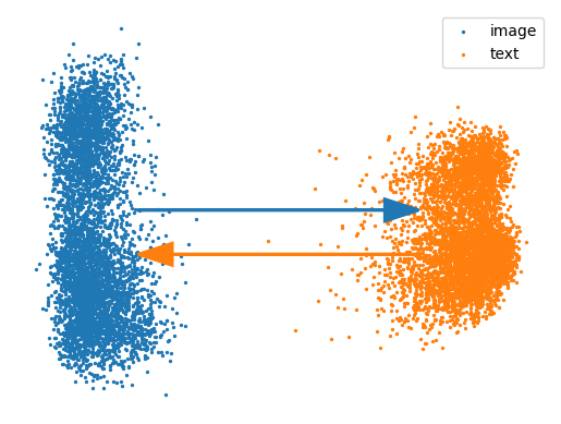
Despite the clear objective that is supposed to bring texts and images to a shared embedding space there is a phenomenon called "Modality Gap" which describes that embeddings of different modalities lie in their own embedding subspaces. The example below visualizes the Modality Gap between images and texts of CLIPWe use the official CLIP implementation by OpenAI: https://github.com/openai/CLIP with the RN50 image encoder. embeddings for a subset of 100 randomly selected images from MSCOCOs validation set. The image and text embeddings are projected to a 2-dimensional space and visualized in a scatter plot. We use a gray line to connect image-text pairs that belong together.

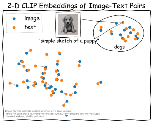
The use of dimensionality reduction methods to compute a 2-dimensional view of the data clearly shows the separation between the two modalities. However, dimensionality reduction comes hand in hand with a loss of information and possible distortion of data. We propose a different way to visualize the dimensionality gap. Similarity heatmaps are a simple yet effective way of visualizing latent space embeddings that also helped us to better understand the modality gap. Using this visualization also allowed us to gain interesting insights unrelated to the modality gap, which we could not have found with the scatter plot visualization alone.

The similarity heatmap below shows the same subset of 100 image-text pairs previously shown in a scatter plot. However, in this case, we show the cosine similaritiesNote that the cosine similarity can yield values between [-1; 1]. calculated between all image and text embeddings. This results in a matrix with four quadrants:

• top-left: in-modal similarities of the 100 image embeddings,
• bottom-right: in-modal similarities of the 100 text embeddings,
• top-right: cross-modal similarities between the 100 image embeddings and the 100 text embeddings,
• bottom-left: a transposed version of the cross-modal image-text similarities.

Now, where does this modality gap even come from?

As analyzed by Liang et al., the modality gap already appears before models are trained, possibly caused by random weight initialization and different model architectures. The authors also highlight that the gap between modalities persists throughout training, which means that CLIP's objective function cannot overcome this phenomenon. A reason for that could be that the objective function only trains on the alignment of (non-)matching image-text combinations but does not contain any regularization terms with regard to the overall layout of the embedding spaces and in-modality alignment. Liang et al. also formally define the modality gap as the Euclidean difference between the centers of each modality:

where x_i and y_i are the normalized image and text embedding vectors.

They also experimented with manually reducing the modality gap by moving the embeddings closer together along the gap vector.

However, since the modality subspaces trained by CLIP are not symmetricGoel et al. argue that the CLIP objective does, in fact, symmetrize the spaces in its optimal solution; in practice however this ideal scenario does not happen. to each other, a modification of the embeddings destroys the complex relationship between images and texts that was derived during training. This naturally results in an increasing loss when changing the distance between modalities that was originally trained, as shown in the visualization below. The x-axis shows the Euclidean distance between the two embedding centers (the black dashed line indicates the original distance). The y-axis shows the contrastive loss that results when moving the two embeddings closer together or further away from each other. We calculated these values with the whole 5000 samples MSCOCO validation set. It becomes visible that the global minimum of this manual intervention is at the point of the original (trained) modality gap.

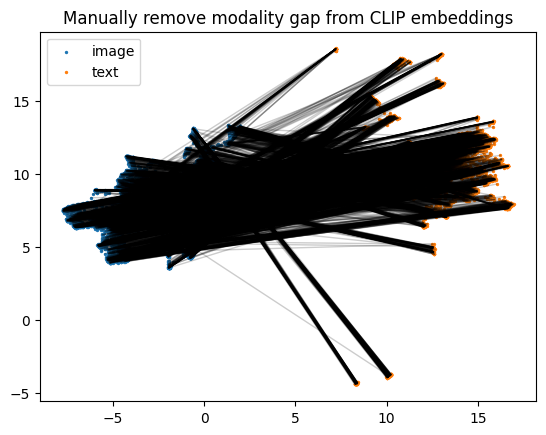
Now, what do the similarity heatmap and scatter plot look like when we manually close the gap? As shown in the visualization below, the similarity matrix seems more homogeneous (i.e., in-modal similarities and cross-modal similarities are on a similar level), and points in the scatter plot are closer together. However, the scatter plot also shows that the edges between image-text pairs are still long, and the text embeddings concentrate more on the center compared to the image embeddings.

What About Other CLIP-Like Models?

As mentioned previously, the two modalities (i.e., texts and images) live on different embedding spaces, and the two embeddings vary in structure (i.e., they are not symmetric to each other). Recently published papers propose different versions of CLIP, where the objective function has been adjusted to regularize the trained embedding space. We look closer into two promising approaches, namely, CyCLIP and CLOOB.

CyCLIP

According to Goel et al. using CLIP-generated image-text embeddings interchangeably (e.g., for Language-guided image generation) is suboptimal because the embeddings are–in practice–not aligned. They propose an augmentation of the InfoNCE loss used to optimize CLIP that adds two regularization terms that enforce the two embedding spaces to be symmetric: one for in-modal symmetry (L_I) and one for cross-modal symmetry (L_C) of the similarities.

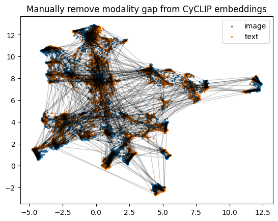
The visualizations below already hint that the embeddings are symmetric: The in-modal similarity heatmaps of the image and text quadrants look similar, and the modalities in the image-text points in the PCA projection seem almost parallel. However, it is also clear that the modality gap is still present.

We can confirm this with a slight modification of the similarity heatmap. For this, we calculate the difference between the in-modal similarities of images and texts, which results in a matrix where values approach zero (i.e., the matrix is a blue rectangle).

When looking back to Liang et al.’s experiments that tried to align the embeddings by moving them along the modality gap vector, we saw that this does not work well for CLIP embeddings because the space is not symmetrized. For CyCLIP, however, the symmetrization is enforced with the objective function, and we could see in the previous plots that the spaces are indeed mostly symmetric. Let's look into the loss landscape for different modality distances of CyCLIP embeddings when moving the embeddings along the gap vector. In the visualization below, we can see that CyCLIP’s loss landscape looks very different from CLIP’s landscape: in the distance interval of [-1.5; 1.5] the loss does not change much, which is another indicator that CyCLIP indeed learns nearly symmetric embedding spacesNote that the loss outside the [-1.5; 1.5] interval increases. This could be due to the fact that the spaces are not perfectly symmetric. Another explanation could be that this happens due to normalizing the embeddings to the unit sphere, but the method proposed for closing the gap is done in Euclidean space..

Again, when closing the modality gap, the similarity heatmap becomes more homogenous (i.e., the in-modal similarities and cross-modal similarities are similarly strong). The image-text pairs in the scatter plot are closer, but still scattered.

Alternatively, we can use UMAP or tSNE projection to better utilize the neighborhoods of similar embeddings instead of linearly determining the axes with the highest variance, as done in PCA. In the case of CyCLIP (scatter plot on the right hand), the use of a neighborhood-based dimensionality reduction technique results in shorter edges and better clustering of similar embeddings. For CLIP (scatter plot on the left hand), edges remain long, and similar images and texts are not clustered together. See the Appendix for examples with 5000 samples.

Let us summarize how the loss changes for CLIP and CyCLIP when moving the embeddings together along the modality gap vector. For that, we again use the entire MSCOCO validation dataset of 5000 samples.

The numbers confirm that CyCLIP's loss changes far less than CLIP's loss when manually closing the gap – it neither gets better nor significantly worse. However, the question arises:

Why Do We Even Want to Close the Modality Gap, if We Do Not Gain Performance?

From a performance optimization point of view, this is a valid question. What's the point of interfering in a well-performing system? On the other hand, the alignment of embedding spaces can become important for other downstream tasks. For example, using image and text embeddings interchangeably, as done in language-guided image generation, relies on the fact that image and text embeddings are aligned with each other and live in the same space. Another aspect is that an aligned embedding space is closer to how humans expect multi-modal models to see the data. Furthermore, closing the modality gap allows us to actually visualize texts and images in the same space, and develop interactive exploration tools that help to understand multi-modal data (e.g., analyzing pairs of human written captions and machine-generated images to find insights about text-to-image generation models like StableDiffusion).

These example use cases of why closing the modality gap might be helpful should give you an incentive about why the pure "performance optimization" point of view is not the only one. In fact, if we can close the modality gap without significantly losing performance, we have a win-win situation!

CLOOB

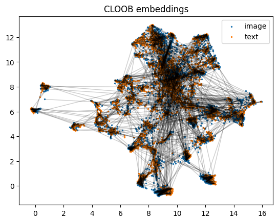
In the previous section, we established a way to manually close the modality gap of CyCLIP embeddings. However, wouldn’t it be better to already close the gap during training and not rely on post-hoc manipulations? While we did not experiment with further modifying (Cy)CLIP’s objective to close the gap during training, we stumbled upon a different learning approach that naturally closes the gap.

Contrastive Leave One Out Boost (short: CLOOB) is a variation of CLIP that proposes an alternative objective together with an associative memory to train the model. The two main components of their method function are (i) modern Hopfield networks and (ii) the InfoLOOB loss instead of the InfoNCE loss used by CLIP. The authors argue that their modifications solve CLIP's "explaining away" problem (i.e., focusing on a small subset of features while ignoring other relevant features) and InfoNCE's saturation problemSee Fürst et al. for more information..

However, we also observe something else: These modifications seem to aid the closure of the modality gap!

We believe that CLOOB’s ability to close the gap during training mainly stems from the cross-modality retrieval applied before calculating the InfoLOOB loss. In this step, the batch of image embeddings and text embeddings is used as an associative memory to create a weighted average of embeddings for the current instance. Since this is done for each combination of embedding and associative memory (i.e., each image and each text embedding is associated with the entire batch of image embeddings AND the entire batch of text embeddings), a stronger correlation between the image/text instances to their own modality and the opposite modality is established. Other influencing factors on closing the modality gap could be the use of InfoLOOB, or the use of modern Hopfield networks that generally have a denoising effectSee this blog post for a detailed explanation of modern hopfield networks: https://ml-jku.github.io/hopfield-layers/..

Summary of Modality Gap Analysis

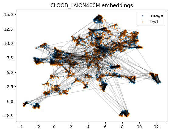
The following visualizations give an overview of the similarity heatmap for CLIP and CyCLIP before (left) and after (right) manually removing the modality gap, as well as the similarity heatmap for CLOOB with the official checkpoints from the paper and a CLOOB version that was trained on the LAION 400M dataset and used a ViT instead of a CNN to encode images. Note how the overall distribution of similarity values differs between the various embedding spaces. For example, the two CLOOB models seem to discriminate more strictly between matching and non-matching image-text pairs.

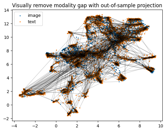
The previous sections taught us about the modality gap, where it comes from, and ways to close it. We also gave reasons for why closing the gap might be beneficial and now demonstrate how closing the modality gap can help with analyzing multi-modal data. We also introduced a handy new way of visualizing latent space embeddings and utilize this again in the following analyses. Finally, we also want to mention that there is a way to visually close the modality gap (i.e., without actually closing the gap in the embedding space), as described in the Appendix.

Converting the Technique into a Tool

Using the previously introduced techniques, we implemented an interactive prototype called “Amumo” (Analyze Multi-Modal Models). Users can switch between models, explore the similarity heatmap and scatter plot visualizations, manually close the modality gap, and try various projection methods.

Identifying Data Subsets

We can look into semantic subsets of data by filtering instances based on their captions. The following example shows the visualizations for the subset that contains the substring "dog". We notice that some lines in the similarity matrix have a darker color. When hovering over those darker lines, we can see that most of these instances correspond to images and texts about "hot dogs" or other images that do not show a dog or where a dog is in an uncommon setting. To make this even more obvious, we can use the "Cluster matrix by similarity" function that reorders the similarity heatmap such that similar lines are grouped together. One cluster that stands out in all three CLIP-like models is the "hot dog" cluster. However, we can also see clusters for "dog and frisbee", "dog and bed", or "dog and car".

Analyze DiffusionDB Dataset

We would like to see what the models’ latent-space embeddings look like for a dataset that is not (entirely) procured by humans. To this end, we use DiffusionDB, a collection of human-written captions and images generated from these captions by Stable Diffusion. We use a subset of 100 randomly selected samples to qualitatively explore the embedding spaces created by the CLIP models we previously introduced. You can use the instance of Amumo below to follow along with the analysis described.

With the default settings, we randomly explore the dataset and get a feeling for the data contained in this subset. We can investigate instances that are outliers in the similarity heatmap by hovering rows or cells that have particularly large or low similarity values. For example, there are some particularly bright cells scattered in the image in-modal similarity heatmap. Upon hovering, we see that all of these images are blurry. We know that DiffusionDB added blur filters for images that were detected to show inappropriate content. Interestingly, CLIP seems to create similar latent embeddings for blurry items, causing them to show high similarity in the similarity heatmap.

For further analyses, we choose "Cluster matrix by similarity" to order the matrix in a way that groups similar rows in the heatmap and investigate the clusters that are emerging. We can see a cluster for "impressionism and crystal" that seems to have homomorphic similarities over all images (i.e., there is a distinct purple line along all images of this cluster). Upon further investigation, we see that the captions in this cluster are mostly vague texts or single words (e.g., "crystal", "impressionism") that can apply to a lot of images. The same cluster becomes apparent in the text in-modal similarity heatmap, where all captions within the cluster seem to have high similarity.

Let’s close the modality gap to investigate clusters in a 2-dimensional scatter plot. We can either do this by switching to the CLOOB model or using CyCLIP in combination with the "Close modality gap" option. We see that the embeddings are aligned and can use the interactive scatter plot to investigate clusters. For example, we can try to find the cluster of blurry images, or we can try to find the cluster with instances of "impressionism". Of course, this would be much more fun on a larger scale :)

Augmentation Analyses

As previously demonstrated, we can identify patterns in datasets and subsets of datasets using the similarity heatmap visualizations. Now, we would also like to see if we can use the same techniques to find patterns in augmentations of a single data point. For example, we take a single image, generate rotated versions of this image, and use this augmented dataset to compute CLIP embeddings and similarities. The results of this experiment for the three CLIP-like models are shown in the visualization below (note that we again show two variants of the CLOOB model). To generate this dataset, we gradually rotate a selected image by 360 degrees over the course of 100 steps. Each step results in a “new” image and a new data point. Note that we only augment the image, but not the text, which results in a completely homogeneous similarity in the in-modal text quadrant of the heatmap and homogenous stripes along the text dimension in the cross-modal quadrants of the heatmap.

When looking at the in-modal image similarity quadrant of the heatmap for each model using augmentations of the first image, we can see an interesting pattern emerge. In addition to the bright yellow diagonal axis that corresponds to the similarities of images to themselves, there is also the perpendicular off-diagonal axis of the matrix sticking out. When hovering along the off-diagonal, we see that the two images along this axis are actually mirrored versions of each other. It seems like all models are invariant to the horizontal flip transformation for this image. We can also see a checkerboard-like pattern emerge for some images emerging in all models except for the CLOOB_LAION400M. When looking into the darker areas of this heatmap in more detail, we can see that the pattern occurs around multiples of 90-degree rotations. The fact that this pattern occurs mainly for the three models that use a CNN-based image encoderNote that CLIP and CLOOB_LAION400M (both 400M instances) were trained on a much larger dataset than CLOOB and CyCLIP, which could also be an indicator for varying robustness. and not for the one with the vision transformer could be an indicator that the two architectures vary in their ability to learn rotation invariant properties. The checkerboard-like pattern seems to be consistent with findings described by Timme et al. where they tested the rotation robustness of various CNN classifiers by measuring the accuracy. The accuracy of the CNNs showed local maxima at multiples of 90-degree rotations and was lower in-between those angles.

When looking at the overall distribution of similarity values, we also notice that the ViT-based CLOOB model seems to have more patches of low-similarity values compared to its CNN-based counterparts. This might indicate that ViT’s overall robustness to rotation transformations is lower. In further investigations, we might want to directly compare two versions of CLIP: the current version with the CNN-based image encoder and a version with a ViT-based image encoder, and study the phenomenon on a larger dataset.

Use the interactions to explore the heatmaps for different images yourself.

In a second experiment, we analyze the heatmaps for an image to which we add an increasingly higher noise level. When looking at the heatmaps for the first image, it seems like there is a certain level of noise for each model, after which the model cannot seem to recognize the content of the image anymore. All images with a higher level of noise than this threshold seem to look (almost) the same (as indicated by a bright yellow rectangle at the lower-right corner of the in-modal image similarity quadrant).

Similarly, for blurry images, we see that at a certain point of blurriness, all images look the same to the models, and they cannot map images and texts together. You can use the dropdown menu to explore the effects of various augmentations.

Conclusion

Throughout this article, we investigated latent embeddings of CLIP-like models. Using scatter plots and similarity heatmaps, we visualized and analyzed the modality gap that naturally occurs for CLIP embeddings. Closing this gap without losing significant performance can be important for downstream tasks like image generation, visual analytics, or human understanding. We showed how to close the gap using CyCLIP in combination with a post-processing method that aligns the embedding spaces and investigated another model (CLOOB) that is able to align the spaces during training. Finally, we introduced Amumo, an interactive visual prototype that allows users to explore embeddings from bi-modal contrastive learning models to help with understanding of their latent space embeddings. We used Amumo to analyze various (sub-)sets and augmentations of data. We believe that Amumo, and the similarity heatmap in particular, are useful tools to create intuition about bi-modal latent space embeddings. It allows for comparison of bi-modal models (e.g., their robustness to transformations) and can help to formulate hypotheses or ideas about such models. However, we want to stress that the analysis is based on a small subset of data points, and insights must still be verified on a larger scale.